What is Logistic Regression?
Logistic regression is basically a supervised classification algorithm. In a classification problem, the target variable(or output), y, can take only discrete values for a given set of features(or inputs), X.
Logistic Regression is generally used for classification purposes. Unlike Linear Regression, the dependent variable can take a limited number of values only i.e, the dependent variable is categorical. When the number of possible outcomes is only two it is called Binary Logistic Regression.
In Linear Regression, the output is the weighted sum of inputs. Logistic Regression is a generalized Linear Regression in the sense that we don’t output the weighted sum of inputs directly, but we pass it through a function that can map any real value between 0 and 1.
In logistic regression, we will use the sigmoid function.
The activation function that is used is known as the sigmoid function. The plot of the sigmoid function looks like.

We can see that the value of the sigmoid function always lies between 0 and 1. The value is exactly 0.5 at X=0. We can use 0.5 as the probability threshold to determine the classes. If the probability is greater than 0.5, we classify it as Class-1(Y=1) or else as Class-0(Y=0).

# imports
import numpy as np
import  matplotlib.pyplot as plt
import pandas as pd
def load_data(path, header):
marks_df = pd.read_csv(path, header=header)
return marks_df
if __name__ == "__main__":

# load the data from the file
data = load_data("data/marks.txt", None)

# X = feature values, all the columns except the last column
X = data.iloc[:, :-1]

# y = target values, last column of the data frame
y = data.iloc[:, -1]

# filter out the applicants that got admitted
admitted = data.loc[y == 1]

# filter out the applicants that din't get admission
not_admitted = data.loc[y == 0]
# plots
plt.scatter(admitted.iloc[:, 0], admitted.iloc[:, 1], s=10, label='Admitted')
plt.scatter(not_admitted.iloc[:, 0], not_admitted.iloc[:, 1], s=10, label='Not Admitted')
plt.legend()
plt.show()
Preparing Data
#Let’s first prepare the data for our model.
X = np.c_[np.ones((X.shape[0], 1)), X]
y = y[:, np.newaxis]
theta = np.zeros((X.shape[1], 1))
We will define some functions that will be used to compute the cost.
#funciton to comppute the cost
def sigmoid(x):
# Activation function used to map any real value between 0 and 1
return 1 / (1 + np.exp(-x))

def net_input(theta, x):
# Computes the weighted sum of inputs
return np.dot(x, theta)

def probability(theta, x):
# Returns the probability after passing through sigmoid
return sigmoid(net_input(theta, x))
Next, we define the cost and the gradient function.
#find the gradient and cost
def cost_function(self, theta, x, y):
# Computes the cost function for all the training samples
    m = x.shape[0]
    total_cost = -(1 / m) * np.sum(
    y * np.log(probability(theta, x)) + (1 - y) * np.log(
    1 - probability(theta, x)))
    return total_cost

def gradient(self, theta, x, y):
# Computes the gradient of the cost function at the point theta
    m = x.shape[0]
    return (1 / m) * np.dot(x.T, sigmoid(net_input(theta, x)) - y)
Fit the Function
Let’s also define the fit function which will be used to find the model parameters that minimize the cost function. In this blog, we coded the gradient descent approach to computing the model parameters. Here, we will use fmin_tnc function from the scipy library. It can be used to compute the minimum for any function. It takes arguments as.
func: the function to minimize
x0: initial values for the parameters that we want to find
fprime: gradient for the function defined by ‘func’.
args: arguments that need to be passed to the functions.
#function to fit x and y
def fit(self, x, y, theta):
  opt_weights = fmin_tnc(func=cost_function, x0=theta,
  fprime=gradient,args=(x, y.flatten()))
  return opt_weights[0]parameters = fit(X, y, theta)
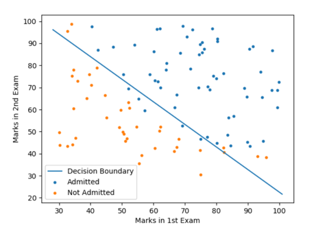
Plotting the decision boundary
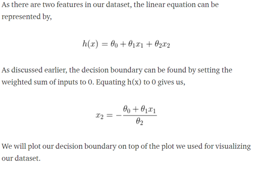
#Ploting the decision boundary
x_values = [np.min(X[:, 1] - 5), np.max(X[:, 2] + 5)]
y_values = - (parameters[0] + np.dot(parameters[1], x_values)) / parameters[2]

plt.plot(x_values, y_values, label='Decision Boundary')
plt.xlabel('Marks in 1st Exam')
plt.ylabel('Marks in 2nd Exam')
plt.legend()
plt.show()
Output:
Accuracy of the model
#Finding the accuracy of model
def predict(self, x):
    theta = parameters[:, np.newaxis]
    return probability(theta, x)def accuracy(self, x, actual_classes, probab_threshold=0.5):
    predicted_classes = (predict(x) >=
                         probab_threshold).astype(int)
    predicted_classes = predicted_classes.flatten()
    accuracy = np.mean(predicted_classes == actual_classes)
    return accuracy * 100accuracy(X, y.flatten())
Implementing Using sklearn
#implement using skleran
from sklearn.linear_model import LogisticRegressionfrom sklearn.metrics import accuracy_score model = LogisticRegression()
model.fit(X, y)
predicted_classes = model.predict(X)
accuracy = accuracy_score(y.flatten(),predicted_classes)
parameters = model.coef_
Get your project or assignment completed by Deep learning expert and experienced developers and researchers.
OR
If you have project files, You can send at codersarts@gmail.com directly