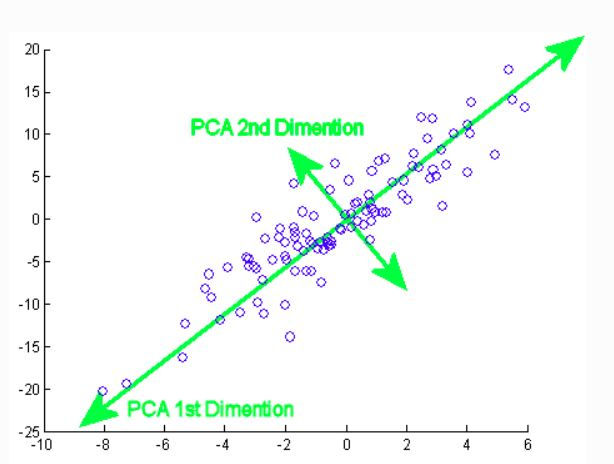
Principal Component Analysis(PCA) In Machine Learning

Principal Component Analysis will help you understand the concepts behind dimensionality reduction and how it can be used to deal with high dimensional data.

Use of principal component analysis

In large dimensional datasets, there might be lots of inconsistencies in the features or lots of redundant features in the dataset, which will only increase the computation time and make data processing and EDA more convoluted.

To solve this problem PCA algorithms are used.

Steps to do this:

• Preparing the data

• Find the covariance matrix

• Calculating the eigenvectors and eigenvalues

• Computing the Principal Components

• Reducing the dimensions of the data set

How to implement it using python

We can implement it using the python, here some steps by which we can implement it.

First importing all the related libraries of PCA.

#Importing all related libraries
from sklearn.decomposition import PCA 
import matplotlib.pyplot as plt 
import seaborn as sns 
import numpy as np 
%matplotlib inline

After this, we load cancer data sets from sklearn:

from sklearn.datasets import load_breast_cancer
cancer = load_breast_cancer()
#show all the keys
cancer.keys()
df = pd.DataFrame(cancer['data'], columns=cancer['feature_names'])
df.head()

After this, we can fit it into the model using below python code:

from sklearn.preprocessing import StandardScaler
scaler  = StandardScaler()
scaler.fit(df)
scaled_data  =  scaler.transform(df)
from sklearn.decomposition import PCA
pca = PCA(n_components =2)
pca.fit(scaled_data)

Output:

PCA(copy=True, iterated_power='auto', n_components=2, random_state=None, svd_solver='auto', tol=0.0, whiten=False)

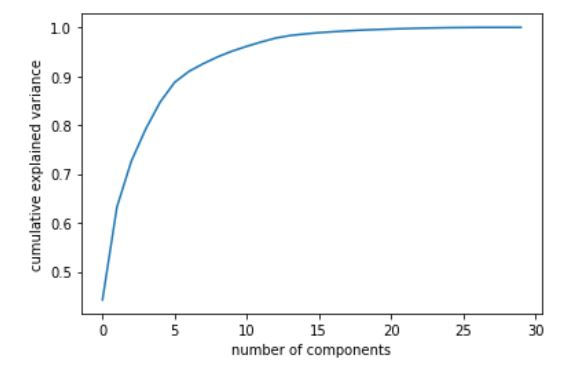
Plot the PCA after reducing the dimension

pca = PCA().fit(scaled_data )
plt.plot(np.cumsum(pca.explained_variance_ratio_))
plt.xlabel('number of components')
plt.ylabel('cumulative explained variance')
plt.show()

The scree plot clearly indicates that the first 500 principal components contain the maximum information (variance) within the data. Note that the initial data set had approximately 9000 features which can now be narrowed down to just 500. Thus, you can now easily perform further analysis on the data since the redundant or insignificant variables are out. This is the power of dimensionality reduction.

Now transform this data into two first principle component:

x_pca = pca.transform(scaled_data)
scaled_data.shape

Output:

(569, 30)

x_pca .shape

Output:

(569, 2)

Good, we are reducing the shape from 30 to 2 dimensions.

Now it is ready to fit into another machine learning model(like linear regression or k-means clustering) to get higher accuracy.

#machinelearning #python #datascience