Beginner's' Guide to Classification using MNIST Fashion Dataset

In deep learning, we use classification algorithms to tackle the problem of identifying objects. One such problem is to train a machine learning model to identify the clothes present in the images. To do this, we will use the MNIST Fashion dataset that consists of the images of clothes. First, we will train the model using the MNIST Fashion dataset, and then we will test the model on new instances of images.

While doing these, you will learn various concepts like normalizing and reshaping the images, and evaluation of the model using a learning curve graph and a confusion matrix.

IMPORT THE ESSENTIAL LIBRARIES

First we will import the libraries to work with.

import warnings
warnings.filterwarnings('ignore')
import pandas as pd
import numpy as np
import matplotlib.pyplot as plt
import matplotlib.image as mpimg
import seaborn as sns

from sklearn.model_selection import train_test_split
from sklearn.metrics import confusion_matrix
import itertools

from keras.utils.np_utils import to_categorical
from keras.models import Sequential
from keras.layers import Dense, Dropout, Flatten, Conv2D, MaxPool2D
from keras.layers import BatchNormalization
from keras.optimizers import RMSprop
from keras.preprocessing.image import ImageDataGenerator
from keras.callbacks import ReduceLROnPlateau

IMPORT THE DATASET

from keras.datasets import fashion_mnist

(X_train, y_train), (X_test, y_test) = fashion_mnist.load_data()

SHAPE OF THE DATASET

print("X_train Shape", X_train.shape)
print("X_test Shape", X_test.shape)
print("y_train Shape", X_train.shape)
print("y_train Shape", X_train.shape)
print("X_train datatype", X_train.dtype)

X_train Shape (60000, 28, 28)
X_test Shape (10000, 28, 28)
y_train Shape (60000, 28, 28)
y_train Shape (60000, 28, 28)
X_train datatype uint8

RESHAPING

Expanding one more dimension for color channel gray

X_train = X_train.reshape(X_train.shape[0], 28, 28,1)
print("X_train Shape", X_train.shape)

X_test = X_test.reshape(X_test.shape[0], 28, 28,1)
print("X_test Shape", X_test.shape)

X_train Shape (60000, 28, 28, 1)
X_test Shape (10000, 28, 28, 1)

clothes = np.array(["T-shirt/top", "Trouser", "Pullover", "Dress", "Coat", "Sandal", "Shirt", "Sneaker", "Bag", "Ankle boot"])

NORMALIZATION

# Normalize the data
X_train = X_train / 255.0
X_test = X_test / 255.0

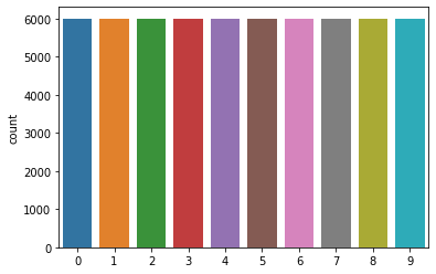
CHECKING DATA IMBALANCE

sns.countplot(y_train)
plt.show()

PERFORMING ONE-HOT ENCODING ON TARGET SET

y_train = to_categorical(y_train, num_classes = 10)
y_test = to_categorical(y_test, num_classes = 10)

DEFINING THE DEEP LEARNING MODEL ARCHITECTURE

def define_model():
    model = Sequential()

    model.add(Conv2D(filters = 32, kernel_size = (5,5),padding = 'Same', 
                    activation ='relu', input_shape = (28,28,1)))
    model.add(BatchNormalization())
    model.add(MaxPool2D(pool_size=(2,2)))
    model.add(BatchNormalization())
    model.add(Dropout(0.25))

    model.add(Conv2D(filters = 64, kernel_size = (3,3),padding = 'Same', 
                    activation ='relu'))
    model.add(BatchNormalization())
    model.add(MaxPool2D(pool_size=(2,2), strides=(2,2)))
    model.add(BatchNormalization())
    model.add(Dropout(0.25))


    model.add(Flatten())
    model.add(Dense(256, activation = "relu"))
    model.add(BatchNormalization())
    model.add(Dropout(0.5))
    model.add(Dense(10, activation = "softmax"))

    return model

LEARNING RATE REDUCTION CONFIGURATION

lr_reduction_config = ReduceLROnPlateau(monitor='val_accuracy', 
                                            patience=3, 
                                            verbose=1, 
                                            factor=0.5, 
                                            min_lr=0.00001)

CREATING A MODEL AND TRAINING THE MODEL

# Fit the model
model = define_model()

model.compile(optimizer = 'adam' , loss = "categorical_crossentropy", metrics=["accuracy"])
history = model.fit(X_train, y_train, epochs=30, validation_split= 5 / 60, batch_size = 64, verbose = 2, callbacks=[lr_reduction_config])

OUTPUT

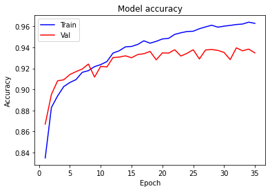
Epoch 1/35 688/688 - 5s - loss: 0.4715 - accuracy: 0.8348 - val_loss: 0.3602 - val_accuracy: 0.8670 - lr: 0.0010 - 5s/epoch - 7ms/step
................................
................................
Epoch 35: ReduceLROnPlateau reducing learning rate to 3.125000148429535e-05. 688/688 - 3s - loss: 0.0992 - accuracy: 0.9629 - val_loss: 0.2015 - val_accuracy: 0.9348 - lr: 6.2500e-05 - 3s/epoch - 5ms/step

EVALUATION OF THE MODEL

# plot accuracy and loss
def plotgraph_accuracy(epochs, acc, val_acc):
    # Plot training & validation accuracy values
    plt.plot(epochs, acc, 'b')
    plt.plot(epochs, val_acc, 'r')
    plt.title('Model accuracy')
    plt.ylabel('Accuracy')
    plt.xlabel('Epoch')
    plt.legend(['Train', 'Val'], loc='upper left')
    plt.show()

# plot accuracy and loss
def plotgraph_loss(epochs, loss, val_loss):
    # Plot training & validation accuracy values
    plt.plot(epochs, loss, 'b')
    plt.plot(epochs, val_loss, 'r')
    plt.title('Model loss')
    plt.ylabel('Loss')
    plt.xlabel('Epoch')
    plt.legend(['Train', 'Val'], loc='upper left')
    plt.show()

# Get the accuracy, loss, and other information
acc = history.history['accuracy']
val_acc = history.history['val_accuracy']
loss = history.history['loss']
val_loss = history.history['val_loss']
epochs = range(1,len(loss)+1)

# Plot the ACCURACY VS EPOCH
plotgraph_accuracy(epochs, acc, val_acc)

# Plot the LOSS VS EPOCH
plotgraph_loss(epochs, loss, val_loss)

model.evaluate(X_test, y_test)

313/313 [==============================] - 1s 3ms/step - loss: 0.2128 - accuracy: 0.9320 
[0.21283283829689026, 0.9319999814033508]

y_pred = np.argmax(model.predict(X_test), axis=-1)

313/313 [==============================] - 1s 2ms/step 

ground_truths = np.argmax(y_test, axis=-1)
cm = confusion_matrix(y_pred, ground_truths)
cmap_value = 'CMRmap_r'
sns.heatmap(cm, annot = True, cmap = cmap_value)
plt.show()

If you are looking for help in any project contact us contact@codersarts.com